Lab 01: Wind Tunnel Characterization

Experiment Overview

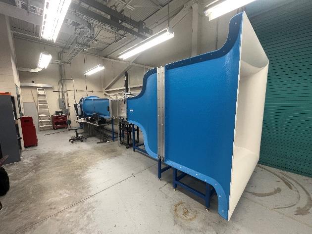
Before any aerodynamic test can be trusted, the wind tunnel itself must be understood. This lab established how the ERAU open-circuit wind tunnel behaves — mapping how fan speed translates to airflow velocity and how that airflow varies across the test section height. These baseline measurements are the foundation every subsequent experiment in the course depends on.

• Operate the ERAU open-circuit wind tunnel and its MATLAB-based data acquisition system
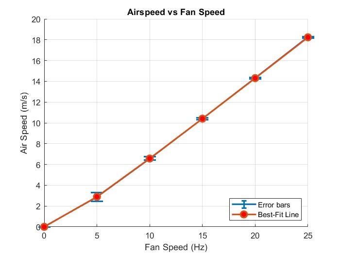
• Quantify how airspeed scales with fan frequency by sweeping 5–25 Hz
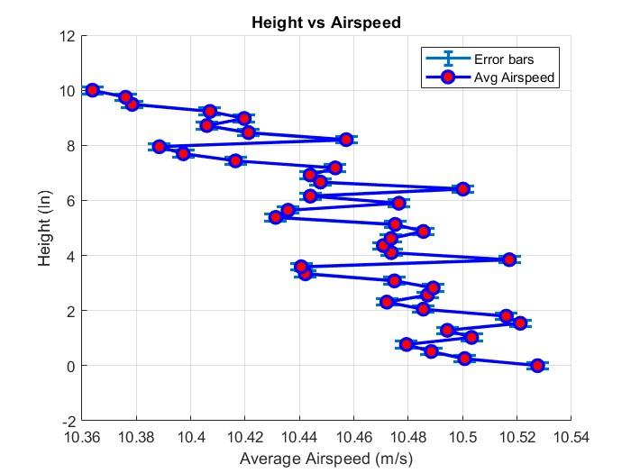
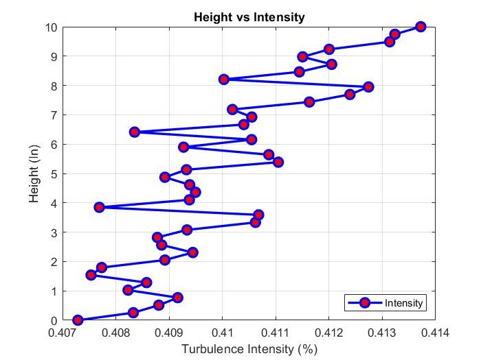
• Profile airspeed and turbulence intensity variation with probe height to assess flow uniformity
• Propagate measurement uncertainty for all recorded velocities using standard error methods

Equipment & Tools

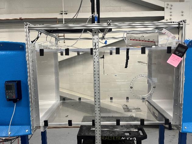
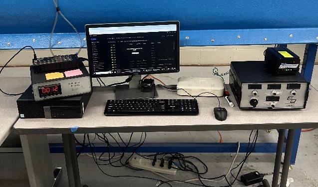
• ERAU open-circuit wind tunnel (inlet, nozzle, test section, diffuser, fan)
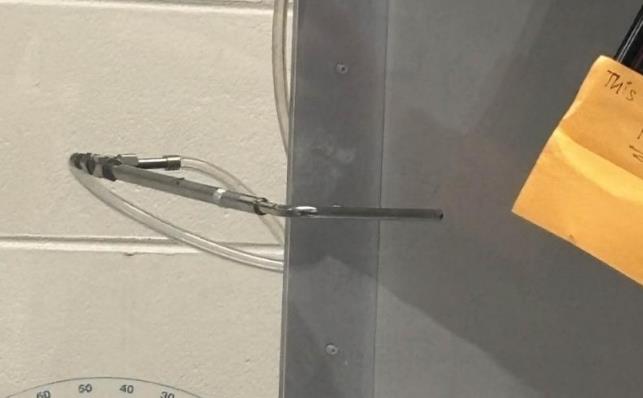
• Traverse pitot-static probe (adjustable height, 1–40 in range)
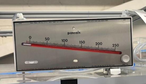
• Analog manometer connected to pitot-static tube
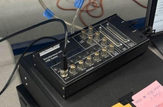
• Analog-to-digital converter (ADC)
• Data acquisition computer with MATLAB DAQ software

Approach & Key Measurements

A traverse pitot-static probe was held at a fixed height while the fan swept from 0 to 25 Hz in 5 Hz steps. Airspeed was computed from the measured differential pressure q using:

V = √(2q / ρ)

where air density ρ was derived from ambient temperature and pressure via the ideal gas law. In a second experiment, the fan was fixed at 15 Hz while the probe traversed 1–40 inches in height. At each position, turbulence intensity I = 100 × σ_V / V̄ was computed to assess flow quality near the tunnel walls. Reynolds number per unit length Re/l = ρV/μ was also recorded at each fan speed, using viscosity from Sutherland’s formula.

Key Results

• Airspeed scaled nearly linearly with fan frequency: 2.89 m/s at 5 Hz up to 18.2 m/s at 25 Hz, validating the tunnel’s controllability across the test range.
• Reynolds number per unit length reached 1.21 × 10⁶ m⁻¹ at 25 Hz, establishing the operating envelope for all subsequent aerodynamic tests in the course.
• Velocity measurement uncertainty dropped from 0.42% at low speeds to 0.056% at 18.2 m/s — higher dynamic pressures yield more accurate airspeed measurements.
• Near the test section ceiling, airspeed decreased slightly and turbulence intensity rose, confirming measurable boundary layer effects that influence test model placement decisions.

MATLAB Code

Differential pressures were loaded from CSV, converted from inches of water to Pascals (×248.84), and used to compute speed and turbulence intensity across both experiments.

% Convert inH2O ? Pa and compute airspeed
Hz_15 = (data(:,4) - data(:,1)) * 248.84;
rho   = 1.213;                              % kg/m³, ideal gas
V_15  = sqrt(2 * Hz_15 / rho);

% Turbulence intensity across probe heights
v_avg     = mean(v, 2);
intensity = (std(v_avg) ./ v_avg) * 100;

% Velocity uncertainty (standard error, %)
UC_V = (std(V_15) / sqrt(length(V_15))) * 100;

Valuable Takeaways

• Calibrating the measurement environment is step one of every test campaign. Understanding the tunnel’s own speed-frequency relationship and cross-section uniformity is essential before trusting any aerodynamic data collected inside it.
• Uncertainty decreases with higher flow speed. Stronger dynamic pressure signals dominate sensor noise, a practical principle that influences how test conditions are selected in both academic and industry wind tunnel programs.
• Wall effects are real and quantifiable. The turbulence intensity rise near the ceiling directly illustrates boundary layer growth, connecting theoretical fluid mechanics to measurement engineering.
• Gained hands-on proficiency with pitot-static probes, analog-to-digital data acquisition, and MATLAB signal processing — all standard tools in aerospace flight test and wind tunnel programs.